Solution to the Jane Street Puzzle of August 2023: Single-Cross 2

In this post, we will solve the Jane Street puzzle of August 2023, which is a probability and calculus problem. To solve it, we will also use a Python script to do some Monte Carlo simulations and symbolic computations. This script can be found in my GitHub.

Statement of the problem

Consider $\R^3$ together with the lattice of unit cubes $\Z^3 \subset \R^3$. For $D > 0$, consider the experiment of choosing a point $A$ (uniformly at random) in the cube $[0, 1]^3 \subset \R^3$, as well as a point $B$ (also uniformly at random) in the sphere centered at $A$ with radius $D$. Let $N$ be the number of times that the line segment $AB$ crosses a face of the cubes in the lattice $\Z^3$ (so, $N$ is a random variable). Question: what is the $D$ that maximizes the probability that $N=1$, and what is that probability?

Probability distribution of $N$ in $\R^1$

For the problem in $\R^3$, define

\[\begin{align*} N_x &\coloneqq \text{number of times the segment crosses a side of a cube along the $x$ axis}, \\ N_y &\coloneqq \text{number of times the segment crosses a side of a cube along the $y$ axis}, \\ N_z &\coloneqq \text{number of times the segment crosses a side of a cube along the $z$ axis}. \end{align*}\]

Then, $N = N_x + N_y + N_z$. As we will later see, this will allow us to reduce the problem in $\R^3$ that we are trying to solve to the analogous problem in $\R^1$.

We will now solve the analogous problem in $\R^1$, for later use. This means that for a length $L$, we choose $x \in [0, 1]$ uniformly at random and we let $N$ be the number of times that the segment $(x, x + L]$ intersects with $\Z$. In other words,

\[\begin{align*} N &= \# \{ n \in \Z \mid x < n \leq x + L \} \\ &= \{ 1, \ldots, \lfloor x + L \rfloor \} \\ &= \lfloor x + L \rfloor. \end{align*}\]

Let $\delta = L - \lfloor L \rfloor$. The previous computation implies that the distribution of $N$ is

\[\begin{align*} P(N = \lfloor L \rfloor) &= 1 - \delta, \\ P(N = \lfloor L \rfloor + 1) &= \delta. \end{align*}\]

Monte Carlo simulation

We now compute $P(N=1)$ for each value of $D$ with a Monte Carlo simulation. This just means that we write some code which repeats the experiment described in the statement of the problem many times to compute the probability. We do not expect such a simulation to give us an extremely accurate result, but Monte Carlo simulations tend to be relatively easy to code and are useful to check if later closed-form results are correct.

The main function of the simulation can be implemented as follows. Here, num_crossings is a function that given the random draw as an input, outputs the corresponding value of $N$. We are using spherical coordinates $\theta \in [0, 2 \pi]$ and $\varphi \in [0, \pi]$.

def prob_one_crossing_mc(d_: float) -> float:
    count = 0

    for _ in range(NUM_EXPERIMENTS):
        # throw segment unif random
        x = uniform(0, 1)
        y = uniform(0, 1)
        z = uniform(0, 1)

        # see https://mathworld.wolfram.com/SpherePointPicking.html
        u = uniform(0, 1)
        v = uniform(0, 1)
        theta = 2 * math.pi * u
        phi = math.acos(2*v - 1)

        # compute num_crossings
        count += 1 == num_crossings(d_, x, y, z, theta, phi)
        
    return count / NUM_EXPERIMENTS

To implement num_crossings, we use the fact that $N = N_x + N_y + N_z$. We separately compute $N_x$, $N_y$ and $N_z$ making calls to a separate function num_crossings_1d.

def num_crossings(
    d_: float, 
    x: float, 
    y: float,
    z: float, 
    theta: float,
    phi: float,
) -> int:
    lx = d_ * math.cos(theta) * math.sin(phi)
    ly = d_ * math.sin(theta) * math.sin(phi)
    lz = d_ * math.cos(phi)
    nx = num_crossings_1d(lx, x)
    ny = num_crossings_1d(ly, y)
    nz = num_crossings_1d(lz, z)
    return nx + ny + nz

In turn, the num_crossings_1d function simply implements the formula $N_{1\mathrm{d}} = \lfloor x + L \rfloor$ that we deduced above (while accounting for the fact that $L_x$, $L_y$, $L_z$ can be negative).

def num_crossings_1d(l: float, x: float) -> int:
    if l < 0:
        l = -l
        x = 1 - x
    return math.floor(x + l)

Running the simulation, we obtain the following plot.

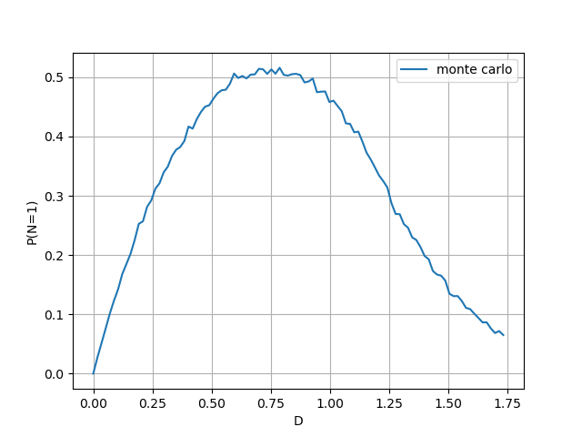
We conclude that the $D$ which maximizes $P(N=1)$ is less than one. In fact, the solution to the problem is approximately $D \simeq 0.75$, $P(N=1) \simeq 0.5$. This means that when deducing a closed-form solution for $P(N=1)$, we may restrict ourselves to the case $D < 1$.

Probability of a single-cross as a function of $D$

Now, we will compute $P(N=1)$ as a function of $D$ (for $D < 1$). Consider the following two experiments: choose $A \in [0, 1]^3$ uniformly at random and then

1. choose a point $B$ in the sphere uniformly at random (this is the same experiment we were already considering);
2. choose a point $B$, uniformly at random, in the region of the sphere corresponding to the spherical coordinates $\theta \in [0, \pi/4]$ and $\varphi \in [0, \pi/2]$.

By symmetry, $N$ has the same distribution in both experiments. This means that for our purposes, we may assume that $\theta \in [0, \pi/4]$ and $\varphi \in [0, \pi/2]$. Let

\[\begin{align*} L_x &= D \cos(\theta) \sin(\varphi), \\ L_y &= D \sin(\theta) \sin(\varphi), \\ L_z &= D \cos(\varphi). \end{align*}\]

Then,

\[\begin{align*} P(N=1) =&\, P(N_x=1, N_y=0, N_z=0) + P(N_x=0, N_y=1, N_z=0) + P(N_x=0, N_y=0, N_z=1) \\ \\ =&\, \hphantom{ {} + {} } \frac{4}{\pi} \int_0^{\pi/4} \int_0^{\pi/2} P(N_x=1, N_y=0, N_z=0 \mid \theta, \varphi) \sin(\varphi) \, \mathrm{d}\varphi \, \mathrm{d}\theta \\ &\, {} + \frac{4}{\pi} \int_0^{\pi/4} \int_0^{\pi/2} P(N_x=0, N_y=1, N_z=0 \mid \theta, \varphi) \sin(\varphi) \, \mathrm{d}\varphi \, \mathrm{d}\theta \\ &\, {} + \frac{4}{\pi} \int_0^{\pi/4} \int_0^{\pi/2} P(N_x=0, N_y=0, N_z=1 \mid \theta, \varphi) \sin(\varphi) \, \mathrm{d}\varphi \, \mathrm{d}\theta \\ \\ =&\, \hphantom{ {} + {} } \frac{4}{\pi} \int_0^{\pi/4} \int_0^{\pi/2} P(N_x=1 \mid \theta, \varphi) P(N_y=0 \mid \theta, \varphi) P(N_z=0 \mid \theta, \varphi) \sin(\varphi) \, \mathrm{d}\varphi \, \mathrm{d}\theta \\ &\, {} + \frac{4}{\pi} \int_0^{\pi/4} \int_0^{\pi/2} P(N_x=0 \mid \theta, \varphi) P(N_y=1 \mid \theta, \varphi) P(N_z=0 \mid \theta, \varphi) \sin(\varphi) \, \mathrm{d}\varphi \, \mathrm{d}\theta \\ &\, {} + \frac{4}{\pi} \int_0^{\pi/4} \int_0^{\pi/2} P(N_x=0 \mid \theta, \varphi) P(N_y=0 \mid \theta, \varphi) P(N_z=1 \mid \theta, \varphi) \sin(\varphi) \, \mathrm{d}\varphi \, \mathrm{d}\theta \\ \\ =&\, \hphantom{ {} + {} } \frac{4}{\pi} \int_0^{\pi/4} \int_0^{\pi/2} L_x (1 - L_y) (1 - L_z) \sin(\varphi) \, \mathrm{d}\varphi \, \mathrm{d}\theta \\ &\, {} + \frac{4}{\pi} \int_0^{\pi/4} \int_0^{\pi/2} (1 - L_x) L_y (1 - L_z) \sin(\varphi) \, \mathrm{d}\varphi \, \mathrm{d}\theta \\ &\, {} + \frac{4}{\pi} \int_0^{\pi/4} \int_0^{\pi/2} (1 - L_x) (1 - L_y) L_z \sin(\varphi) \, \mathrm{d}\varphi \, \mathrm{d}\theta \\ \end{align*}\]

Here, in the first equality we used $N = N_x + N_y + N_z$, in the second we used the law of total probability, in the third we used the fact that for fixed $\theta$, $\varphi$, the events ${N_x=i, N_y=j, N_z=k}$ are independent, and in the fourth we used the computation in $\R^1$ from above (with $D \leq 1$).

To obtain a formula for $P(N=1)$, we will use the Python symbolic calculus library SymPy. The following code computes the integrals above:

d, th, ph = symbols('d th ph')

lx = d * cos(th) * sin(ph)
ly = d * sin(th) * sin(ph)
lz = d * cos(ph)

IX = lx * (1 - ly) * (1 - lz) 
IY = (1 - lx) * ly * (1 - lz)
IZ = (1 - lx) * (1 - ly) * lz
I = IX + IY + IZ

p = (4/pi) * integrate(integrate(I * sin(ph), (ph, 0, pi/2)), (th, 0, pi/4))
p = p.simplify()

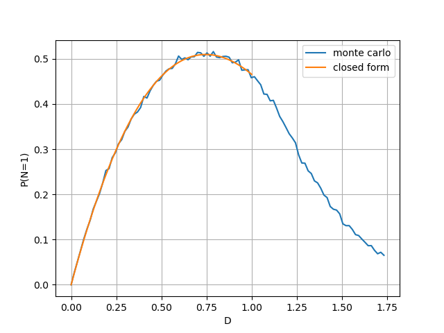
Denoting $p(D) = P(N=1)$, the output of the Python script tells us that

\[p(D) = \frac{1}{4\pi} D (3 D^2 - 16 D + 6 \pi) \qquad (\text{if $D \leq 1$}).\]

The figure below shows that this formula gives the same result as the Monte Carlo simulation.

Optimization of $p(D)$

To find $D$ which maximizes $p(D)$, we compute the derivative $p^\prime(D)$:

\[p^\prime(D) = \frac{1}{4\pi} (9 D^2 - 32 D + 6 \pi)\]

The equation $p^\prime(D) = 0$ has a unique solution in $[0, 1]$, which is

\[\begin{align*} D &= \frac{1}{9} (16 - \sqrt{256 - 54 \pi}) = 0.7452572091, \\ p(D) &= \frac{8}{3} - \frac{2048}{243 \pi} + \left( \frac{128}{243 \pi} - \frac{1}{9} \right) \sqrt{256 - 54 \pi} = 0.5095346021. \end{align*}\]